In this post, I will dwell on something essential to the success of any decision-making.
How to measure the success of a given decision?
To measure the success of a given decision, businesses can use various metrics and key performance indicators (KPIs) to track the effectiveness of their decisions. It’s important to choose the right metrics that align with your business goals and use them consistently over time to measure progress and identify areas for improvement.
Particularly,
Let’s assume you are a driven entrepreneur optimizing every cent you are spending to get the best of the best outcome. For instance, you are running a marketing campaign on various channels such as Social Media, Flyers, Radio, etc. And one can also assume that your main concern at this point is to raise the revenue as much as possible with spending on advertisements on different channels. How can you know the most effective channels that generates revenue for your business?
MMM
Media Mix Modeling (MMM) is a marketing approach that models the effects of different channels on sales. MMM problems involve channel-specific effects like delays, saturation, and long-term effects that are modeled through different parameters. Classical MMMs require assumptions about media channel behavior to assess each channel’s contribution to sales through linear regression.
The Bayesian MMM approach offers an all-in-one estimation of both channel behavior and sales lift through prior distributions and data. MMM involves nonlinear transformations such as saturation and time-delay. The aim of incorporating nonlinear transformations to marketing investment features is to capture the anticipated actions from media channels that cannot be represented through linear mappings.
By utilizing the Bayesian approach, it is possible to estimate all the parameters (both regression and nonlinear interaction) in a single model, which can incorporate information as prior knowledge to achieve optimal performance even when there is a lack of data. This approach avoids incorrect and unchangeable assumptions if past channel-specific studies were not performed. Qualitative and quantitative business knowledge can be translated into tailored prior distributions to optimize the model’s performance. Prior knowledge can be included as prior distributions to help the model find a sensible parameter combination.
Choosing the prior distribution for the parameters can be seen as your prior belief regarding to effect on the target. If you are not sure of the impact on the target variable, you can feed it an uninformed prior (e.g. the standard normal distribution) for that variable and let the model learn it by itself.
Model
This work is based on Jin, Yuxue, et al (2017) in which they provided a Bayesian mixed media model with carryover and shape effect. I avoided modeling ad stock shape effects with saturation or diminishing returns. For the sake of completeness, I will define the problem:
$y_{t} = \tau + \sum_{m=1}^{M} \beta_{m} f(x_{t,m};w) + \sum_{c=1}^{C} \gamma_{c}z_{t,c}+\epsilon_{t}$
Time series data with $y$ target variable (revenue), channel spending $x$ and control variables $z$ captures trend and seasonality. In time period $t = 1 \dots T$. There are $M$ media channels in the media mix, and $x_{t,m}$ is the media spend of channel $m$ at week $t$ It is considered a linear model of the form where $\tau$ is the intercept capturing baseline sales, and $\epsilon$ capturing noise is assumed to be uncorrelated with other variables and have constant variance. $f$ is the ad stock function:
$f(x,w_{m},L) = \frac{\sum_{l=0}^{L-1} w_m(l;\alpha_{m},\theta_{m}) x_{t-l,m}}{\sum_{l=0}^{L-1} w_m(l)}$
$w_m(l,\alpha_m,\theta_m)=\alpha_{m}^{(l-\theta_m)^2}$
Ad stock function takes as input media spends for a given media during L weeks, the retain-rate and the delay of the peak. The delay is the number of periods before the peak effect. The ad stock function is responsible for capturing the temporal effects of diverse advertising channels. $\alpha_{m}$ representing the retention rate of ad effect and $\theta_{m}$ represents the delay in the peak effect of the $m$-th channel. $L$ is the maximum time period that delay can incur effect and it is set to be 13.
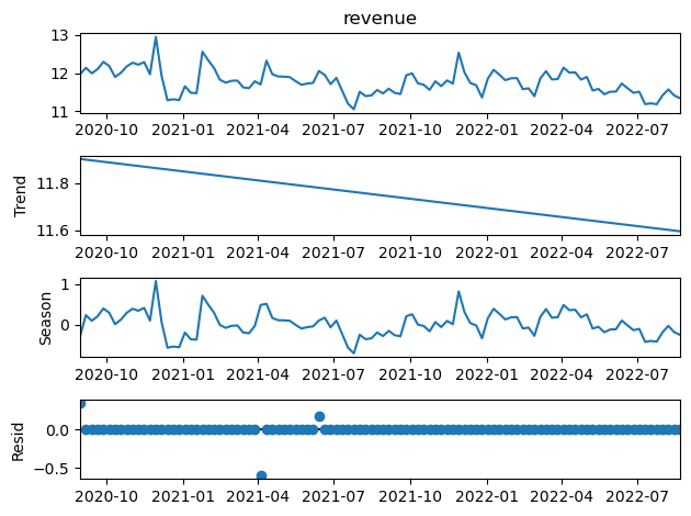
Seasonality and Trend
Employing Seasonal-Trend decomposition using LOWESS (locally estimated weighted scatterplot smoothing). For log of target value and setting seasonal to 7 results in lowest residual. This supports the need of additive modeling of seasonality and trend. The idea is to make a matrix of Fourier features which get multiplied by a vector of coefficients to to capture the seasonality. Number of order to create fourier pairs will be 7 (14 new features). Trend will be modeled as linear function.
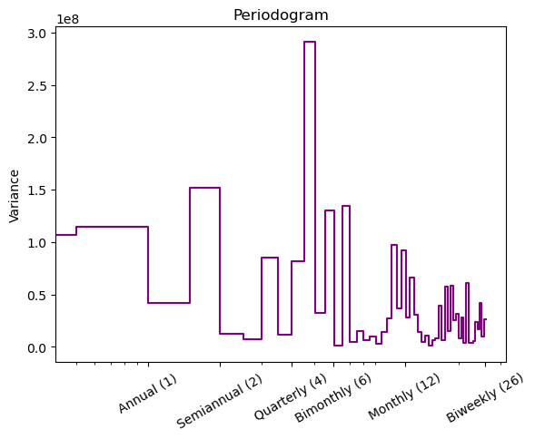
This is further supported by a periodogram where drop after bi-monthly can be seen from the figure below.
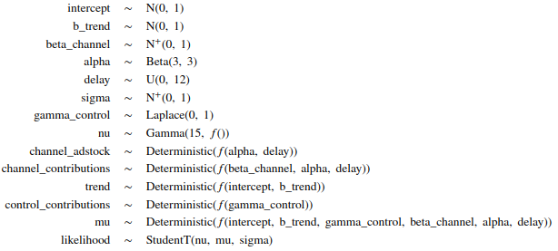
Likelihood and Prior distributions
The prior distribution represents the beliefs or assumptions you have about the variables before analyzing the data. Starting point for the choice of priors is following the work done by Jin, Yuxue, et al (2017). Parameter optimization is avoided for now but one can further it using Bayesian model selection criteria. $\alpha \backsim Beta(3,3)$, $\theta \backsim Uniform(0,12)$, $\gamma \backsim Laplace(0,1)$ for the fourier coefficient to add certain regularization, $\tau \backsim Normal(0,1)$ additionally trend has a coefficient with $~Normal(0,1)$
I use a $HalfNormal(1)$ distribution for the media coefficients to ensure they are positive.
The likelihood function describes the relationship between the data and the parameters of the model. Choosing an appropriate likelihood function is critical to accurately model the data. Main model I used for the likelihood function is a StudentT distribution which is robust against outliers as suggested by [4] with the precision prior parameter $\nu \backsim Gamme(15,1)$. It is suggested by [4] to use MaxAbsScaler which is convenient to use due to transformation while calculation ROAS.
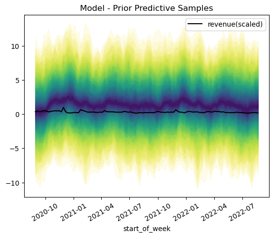
Model validation
Prior predictive checks make use of simulations from the model. Range is limited to but suggesting negative revenue especially in the initial points should be investigated further. Additional data to support initiation could be effective.
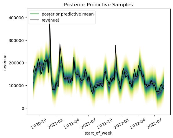
It is important to validate the model to ensure that it is reliable and accurate. This can be done by by using posterior predictive checks. Posterior predictive checking also allows one to examine the fit of a model to real data. We see that some extreme values can not be captured.
Channel performance
Channel 3 , Channel 7, Channel 6 contributions are highest to revenue. It is followed by Channel 4, Channel 5. Lowest contributions are from Channel 2, Channel 1 (see notebook) Further we observe that delay parameters have high HDI range and fail to converge. This could further improved by using saturation function. We also observe that the Channel 3 (coeff =0.376), Channel 7 (coeff = 320) and Channel 6 (coeff =305 ) has highest average contribution by unit spending. It is followed by Channel 2( coeff = (0.225))
Model Comparison
We can check the difference with respect to using normal distributed likelihood. To evaluate model performance and to measure it we will use Pareto smoothed importance sampling leave-one-out cross-validation (LOO). We see that our initial model performs better.
Further diagnostics can be applied by checking residuals of the model. For each MCMC draw of posterior samples of the parameters we should compute autocorrelation of the residuals of the regression model as suggested by[1] Since this is our main model assumption.
github repo: https://github.com/alpertaskiran/bayesian_mmm TODO: compute autocorrelation of residuals, implement ROAS
References:
[2] Gelman, Andrew, et al. “Bayesian Workflow.” ArXiv.org, 3 Nov. 2020
[3] PyMC-Marketing : https://github.com/pymc-labs/pymc-marketing
[4] Media effect estimation with pymc: Adstock, saturation & diminishing returns. Dr. Juan Camilo Orduz. (2022, February 11). Retrieved April 17, 2023, from https://juanitorduz.github.io/pymc_mmm/